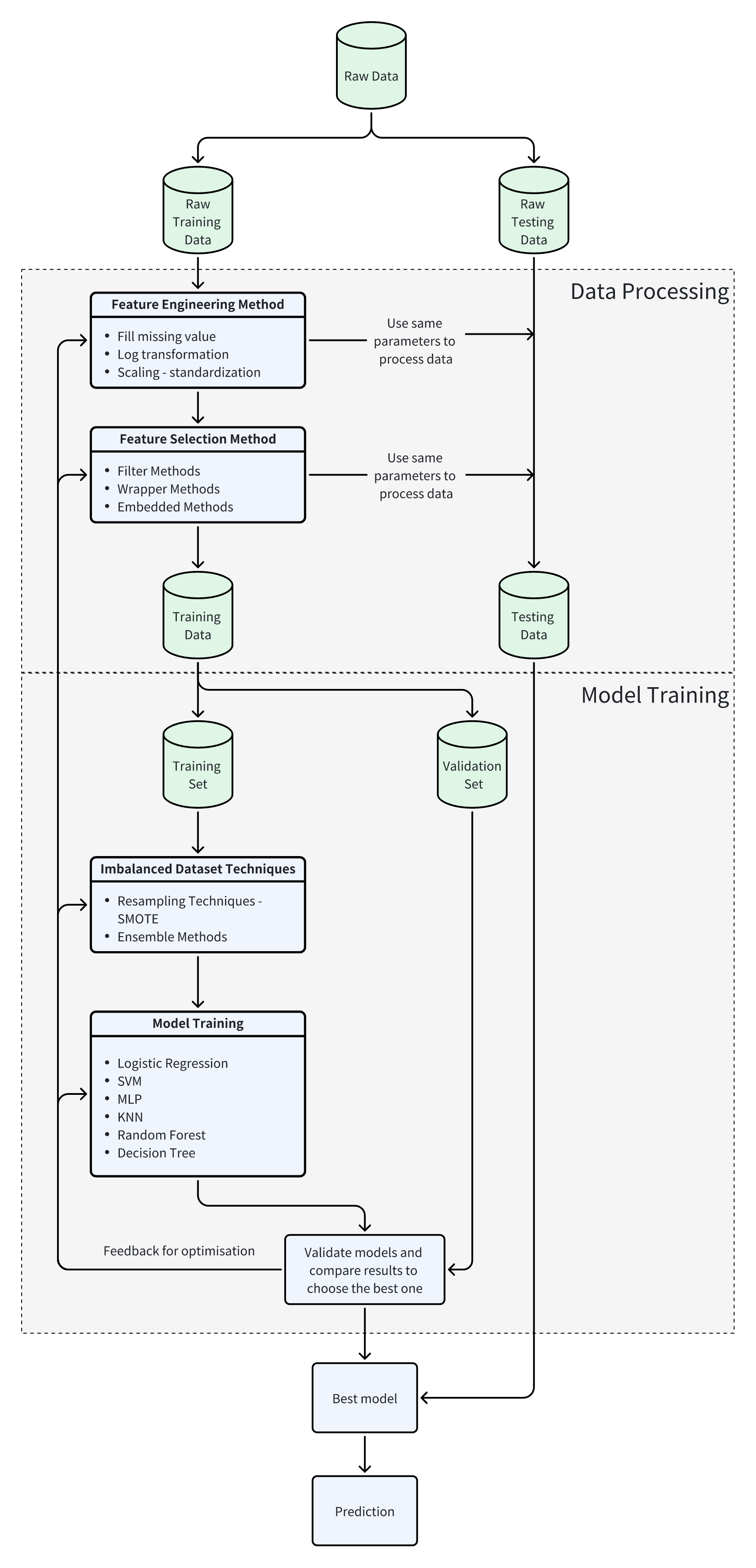
Rail Break Prediction AI project focuses on building a data pipeline to extract, enrich, and analyse real-world data using machine learning models, with the goal of predicting rail breaks within the coming 30 days, utilising the Insight Factory platform.
Software Architecture
Images
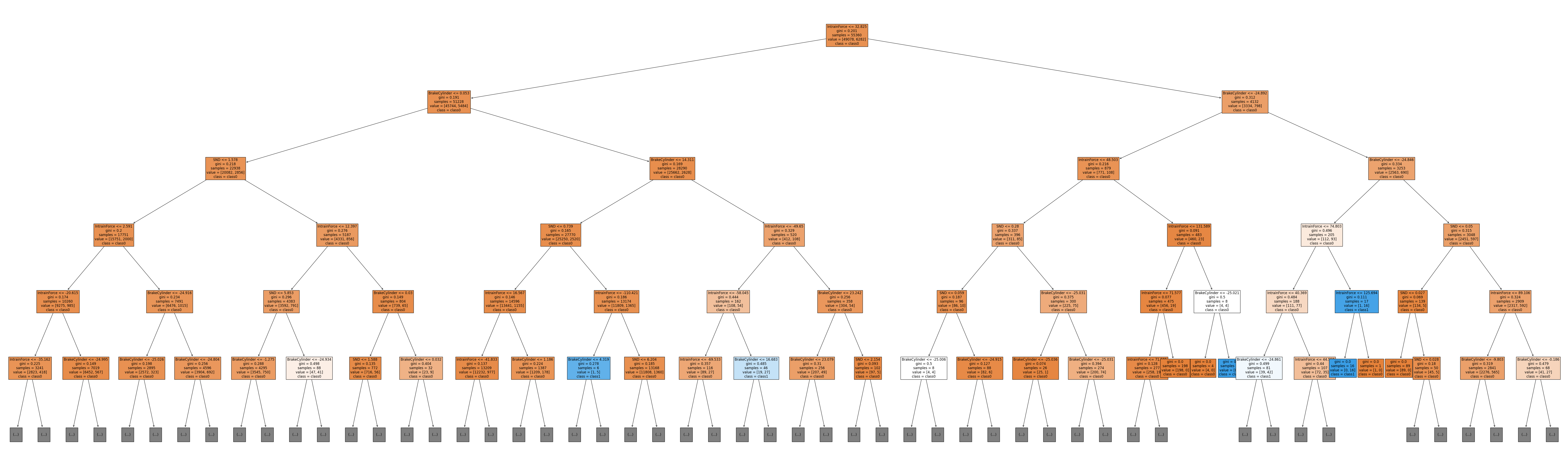
Code - XAI of Decision Tree
0 - data and train
df = spark.sql("""select * from demo.training_table""")
df = df.fillna(0)
# select data
feature_columns = ['BrakeCylinder', 'IntrainForce', 'SND']
target_column = 'target'
# 提取 X 和 y 在 PySpark 中
X = df.select(feature_columns).toPandas()
y = df.select(target_column).toPandas()

print(X.columns)
print(y.columns)
from sklearn.tree import DecisionTreeClassifier
from sklearn.model_selection import train_test_split
from sklearn.metrics import accuracy_score, f1_score

# Split the data into training and testing sets
X_train, X_test, y_train, y_test = train_test_split(X, y, test_size=0.2, random_state=42)

# 2. create a tree classifier
clf = DecisionTreeClassifier()

# 3. train
clf.fit(X_train, y_train)

# 4. predict
y_pred = clf.predict(X_test)

# 5. get accuracy
accuracy = accuracy_score(y_test, y_pred)
print(f"Accuracy: {accuracy}")

# F1 score
f1 = f1_score(y_test, y_pred, average='binary')
	# You can also use 'micro' or 'macro' or 'weighted' depending on your need
print(f"F1 Score: {f1}")

true_positive = 0
true_negative = 0
false_positive = 0
false_negative = 0
for i in range(len(y_pred)):
    pred = y_pred[i] != 0
    real = y_test.iloc[i][0] != 0
    # if y_pred[i] != 0 or y_test.iloc[i][0] != 0:
        # print(y_pred[i], y_test.iloc[i][0])
    if pred == 0 and real == 0:
        true_negative += 1
    elif pred == real == 1:
        true_positive += 1
    elif pred == 0 and real == 1:
        false_negative += 1
    elif pred == 1 and real == 0:
        false_positive += 1
print("true positive = ", true_positive)
print("true negative = ", true_negative)
print("false positive = ", false_positive)
print("false negative = ", false_positive)
precision = true_positive / (true_positive + false_positive)
recall = true_positive / (true_positive + false_negative)
print("precision = ", precision)
print("recall = ", recall)
print("f1 = ", precision * recall * 2 / (precision + recall))
print("my percision = ", true_positive / (true_positive + false_positive + false_negative))
# control center
class_number = clf.n_classes_
feature_number = clf.n_features_in_
print(f"class number   = {class_number} -> {clf.classes_}")
print(f"feature number = {feature_number}")

# decision tree model = clf
class_names = [f"class{i}" for i in range(class_number)]  # 2 class
# feature_names = [str(i) for i in range(feature_number)]  # 3 feature
feature_names = ['BrakeCylinder', 'IntrainForce', 'SND']
1 - visualise tree
from sklearn.tree import DecisionTreeClassifier
from sklearn import tree
import matplotlib.pyplot as plt

# visualise decision tree
temp = plt.figure(figsize=(100, 30))
temp = tree.plot_tree(clf, feature_names=feature_names, class_names=class_names, filled=True, max_depth=5, fontsize=12)
plt.show()
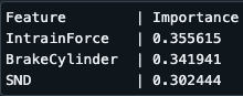
2 - Feature Importance
import numpy as np

# Get Feature Importance
importances = clf.feature_importances_

# Match feature name and Importance
# feature_names = [str(i) for i in range(3)]
feature_importances = sorted(zip(feature_names, importances), key=lambda x: x[1], reverse=True)

# Print the top 10 most important features
print(f"Feature        | Importance")
for feature, importance in feature_importances[:10]:
    print(f"{feature:15}| {importance:.6f}")
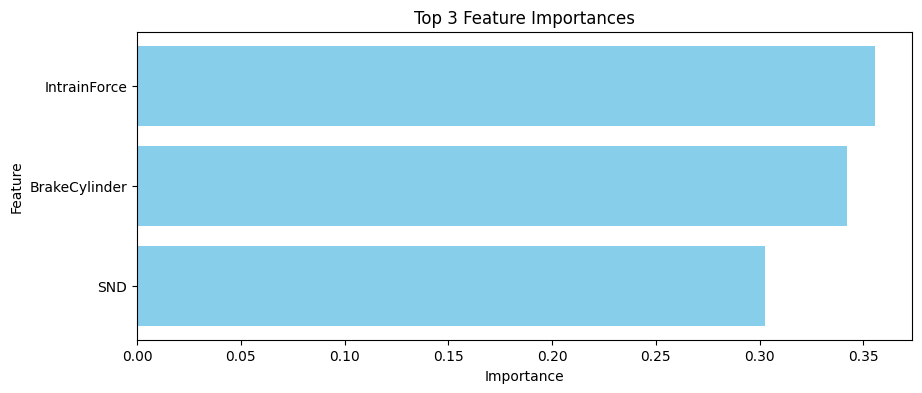
import matplotlib.pyplot as plt

# Select the top 20 most important features for visualization
top_n = 20
top_features = [f[0] for f in feature_importances[:top_n]]
top_importances = [f[1] for f in feature_importances[:top_n]]

# Plot figure
plt.figure(figsize=(10, 4))
plt.barh(top_features, top_importances, color='skyblue')
plt.xlabel('Importance')
plt.ylabel('Feature')
plt.title(f'Top {len(top_features)} Feature Importances')
plt.gca().invert_yaxis()  # Features are listed from highest to lowest
plt.show()
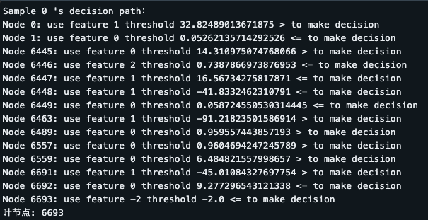
3 - Decision Path
import numpy as np
from sklearn.tree import DecisionTreeClassifier
from sklearn import tree
import matplotlib.pyplot as plt

# Choose a sample by index
sample_index = 0
X_sample = X_test.iloc[sample_index].to_numpy().reshape(1, -1)

# get decision path
decision_path = clf.decision_path(X_sample)

# Prints the index of the node passed on the path
node_indicator = decision_path[0]
leaf_id = clf.apply(X_sample)

# print decision path
print(f"Sample {sample_index} 's decision path:")
for node_id in node_indicator.indices:
    # Print the feature number and threshold
    if node_id in clf.tree_.children_left:
        threshold_sign = "<="
    else:
        threshold_sign = ">"

    print(f"Node {node_id}: use feature {clf.tree_.feature[node_id]} threshold {clf.tree_.threshold[node_id]} {threshold_sign} to make decision")

# The last node is the leaf node
print(f"Leaf Node: {leaf_id[0]}")
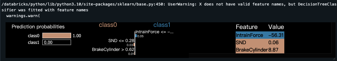
4 - LIME
import lime
import lime.lime_tabular
import numpy as np

# Ensure X_train and X_test are numpy arrays
X_train = np.array(X_train)
X_test = np.array(X_test)

# model is clf, traning set is X_test
explainer = lime.lime_tabular.LimeTabularExplainer(X_train, feature_names=feature_names, class_names=class_names, discretize_continuous=True)

# choose a sample
i = 0
exp = explainer.explain_instance(X_test[i], clf.predict_proba, num_features=10)

# show result
exp.show_in_notebook(show_all=False)